Farr, M.T., Green, D.S., Holekamp, K.E., Roloff, G.J., and Zipkin, E.F. (In Press) Multispecies hierarchical modeling reveals variable responses of African carnivores to management alternatives. Ecological Applications.
Description
This work was done with Dr. David Green, Dr. Kay Holekamp, Dr. Gary Roloff, and my advisor Dr. Elise Zipkin to quantify the impact of anthropogenic disturbance and management alternatives on the carnivore community within the Masai Mara National Reserve (MMNR), Kenya. Carnivore communities in the Serengeti-Mara ecosystem, including the MMNR, are among the most diverse in the world, but human-wildlife conflict threatens the continuation of this community. To understand the impact of anthropogenic disturbance on the carnivore community, we compared two disparate management regions within the MMNR that are managed by separate entities. The Mara Triangle experiences minimal disturbance while the Talek region contains high frequency of human-wildlife conflict. Using a hierarchical multispecies distance sampling model we estimated the community wide and species-specific effects of the Talek region on carnivore abundance and compared species abundances and group sizes between regions.
Background
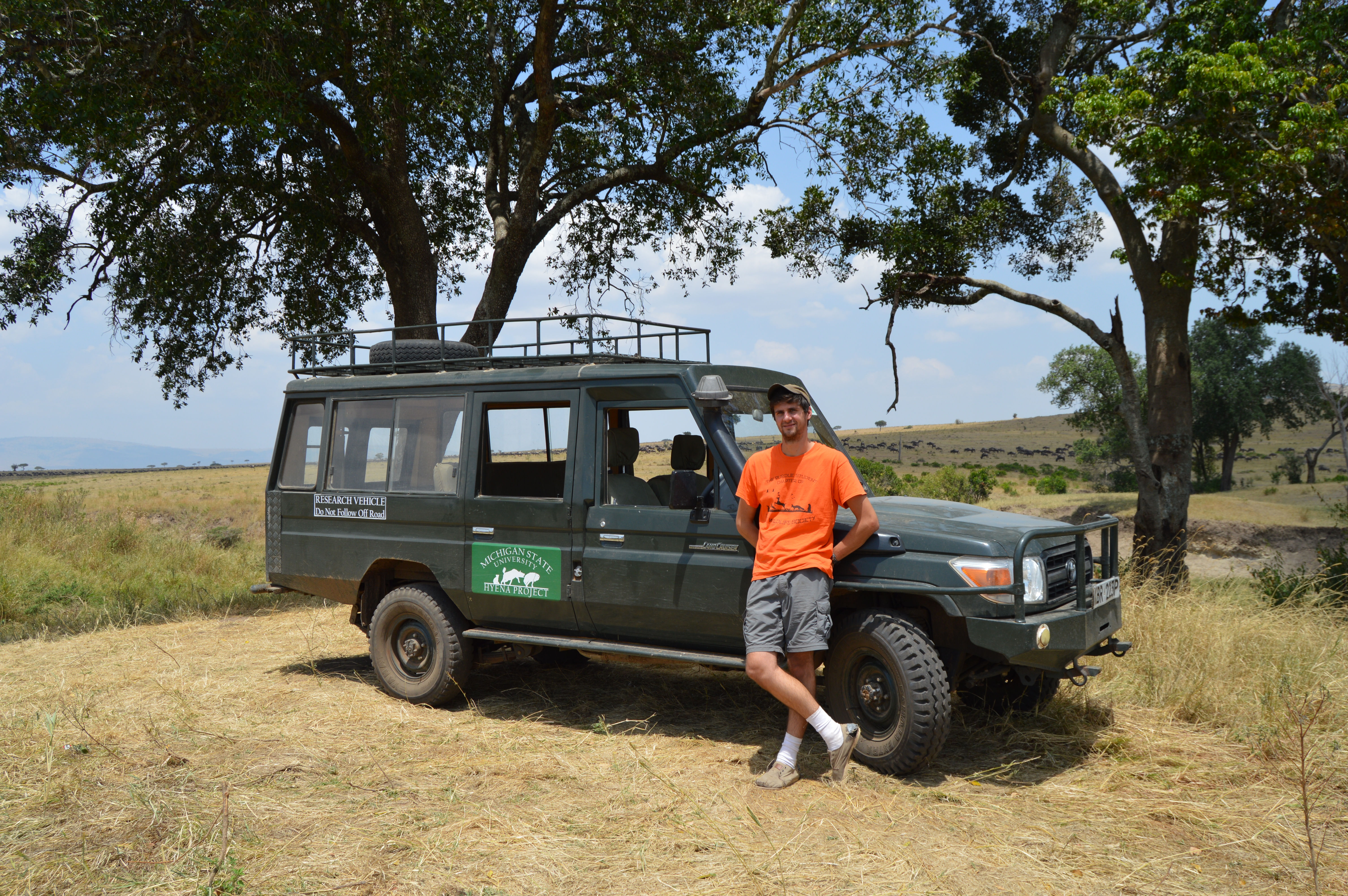
This was my first project as a graduate student, but the idea for this research originated before I started at Michigan State University (MSU). My part in this project began when I visited MSU as a prospective student for the Zipkin Quantitative Ecology Lab. Elise encouraged me to talk with members of her department where I met Kay for the first time. At the time I was finishing a job as a field technician and looking for work. Coincidently, Kay was in need of a technician for her Mara Hyena Project. In less than a month I was on a plane headed to Nairobi, Kenya to begin an 8 month adventure in the Masai Mara National Reserve.

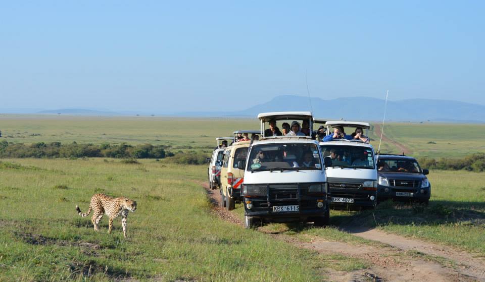
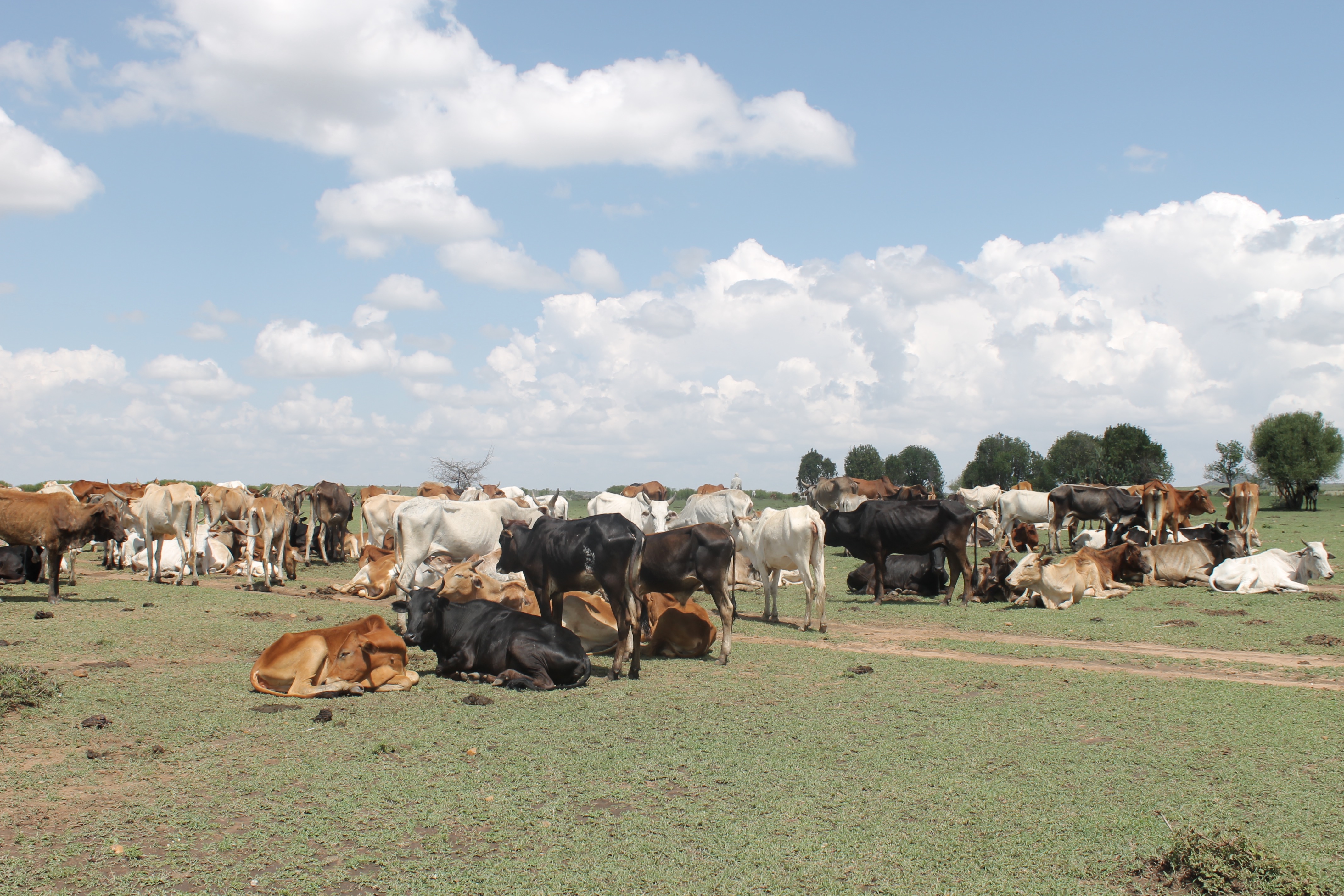
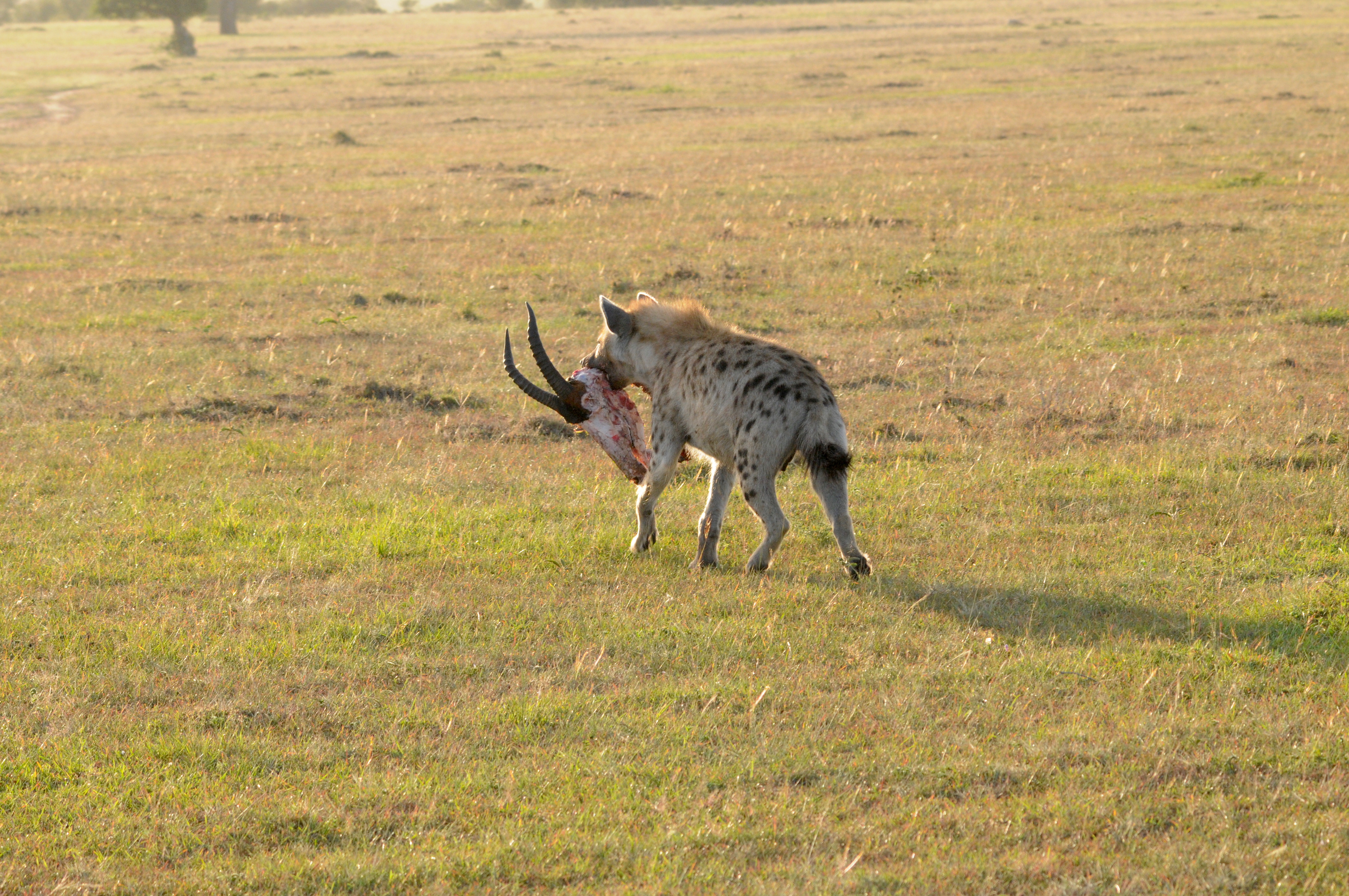
Prior to my departure, Elise and I discussed the possiblility of using long-term data from Kay’s project for my dissertation research. So while I was primarily working on Kay’s project (monitoring the behavioral ecology of spotted hyenas), I was also keeping my eyes open for a potential interesting research question. During my tenure there, nothing was more obvious than the intensity of human disturbance in the form of tourism and livestock grazing. We counted over 10,000 cows, sheep, and goats in a single night! And too many times to remember we observed hyenas taking advantage of an easy steak dinner.
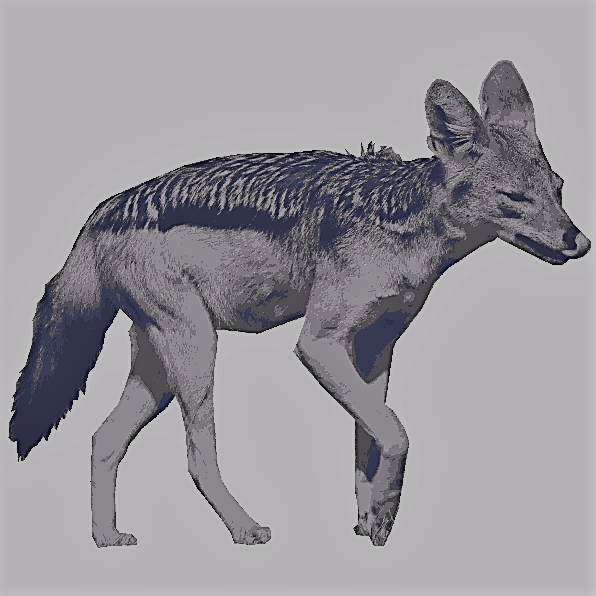
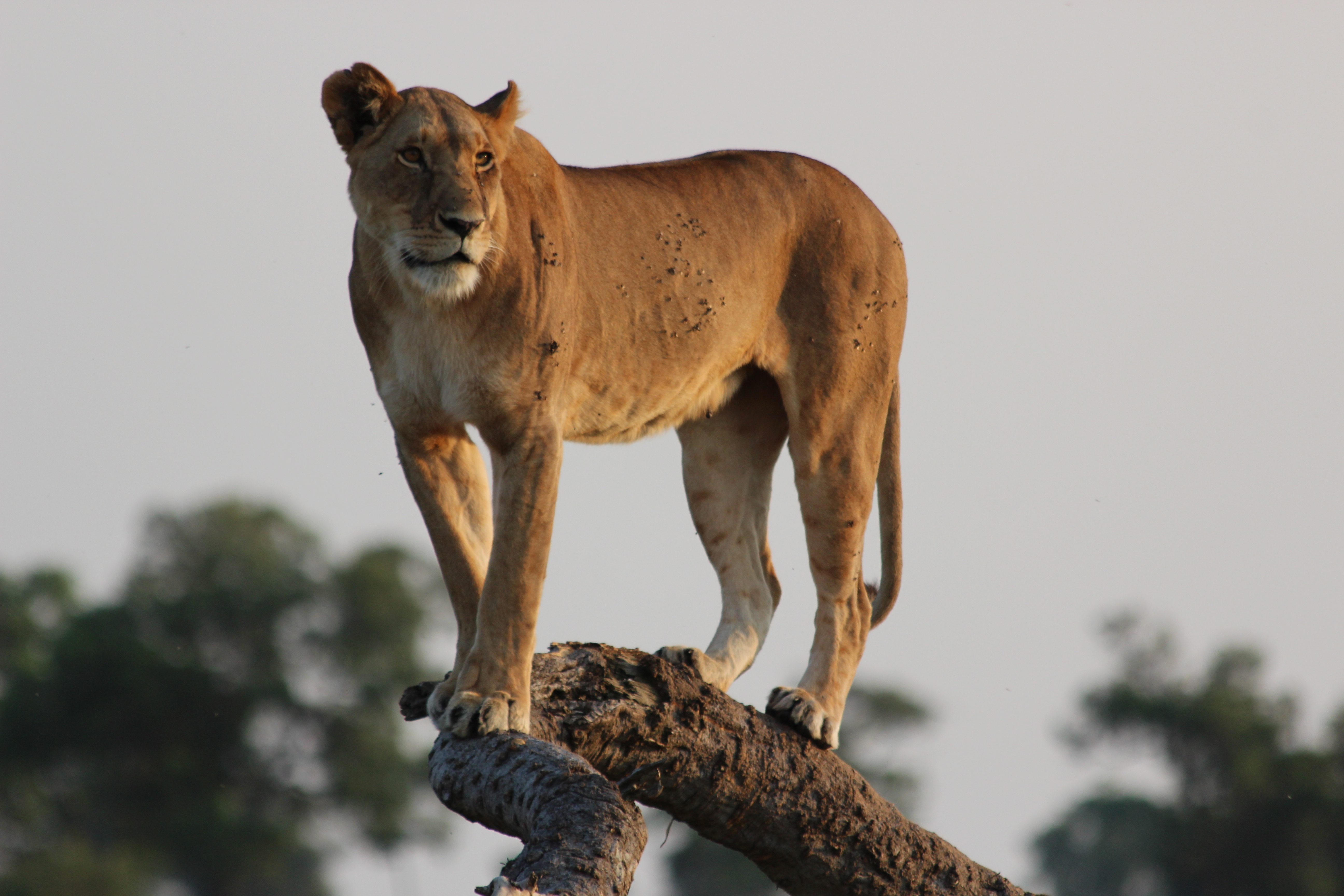
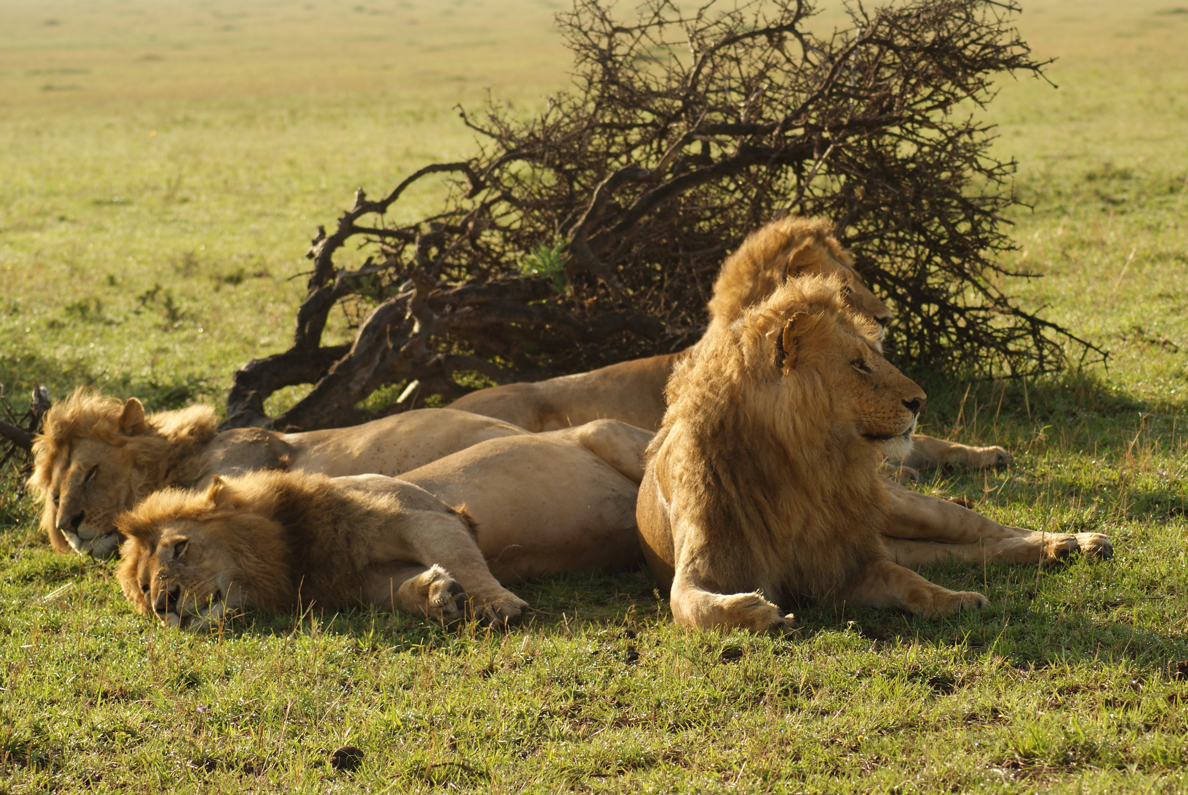
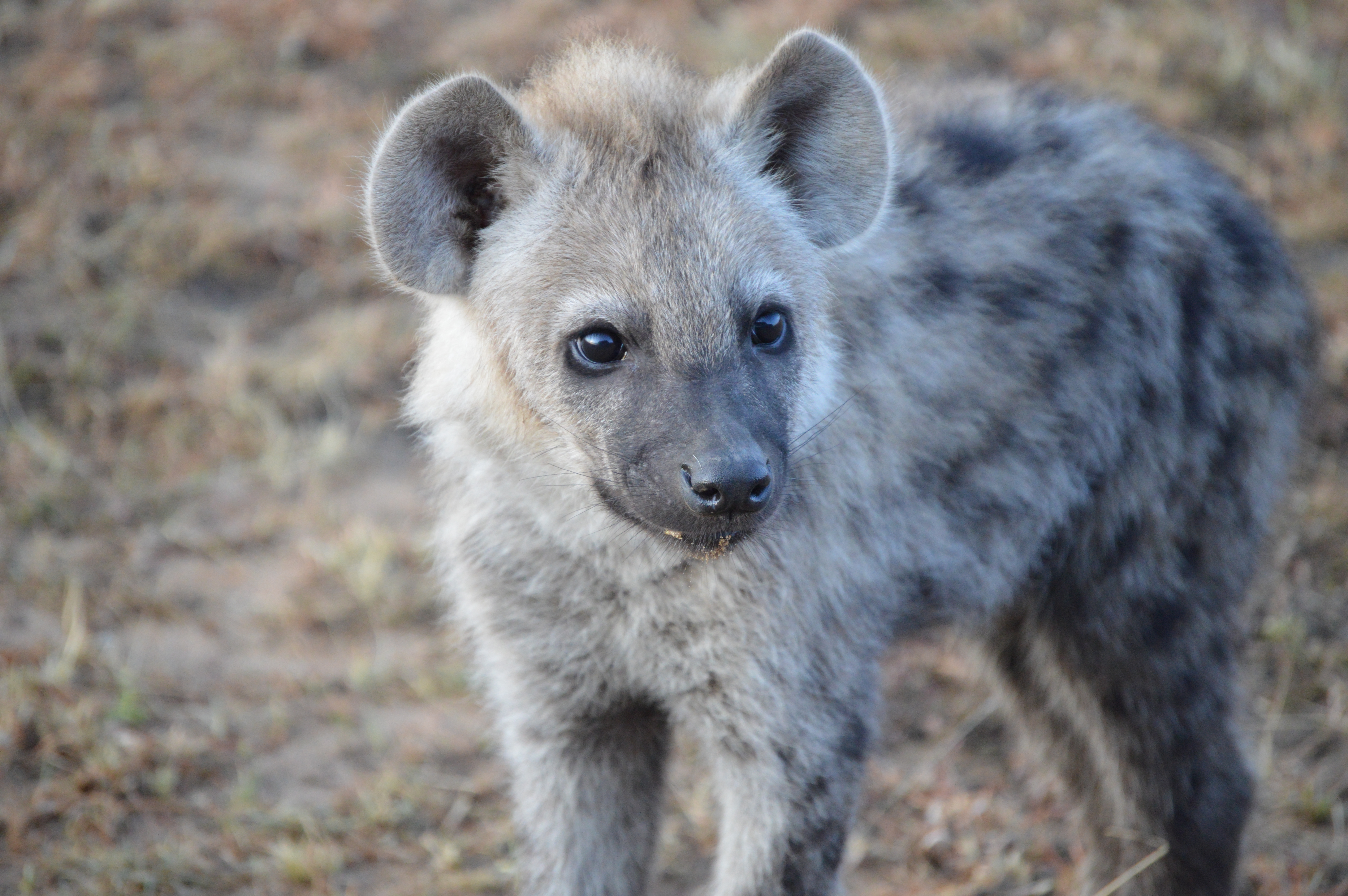
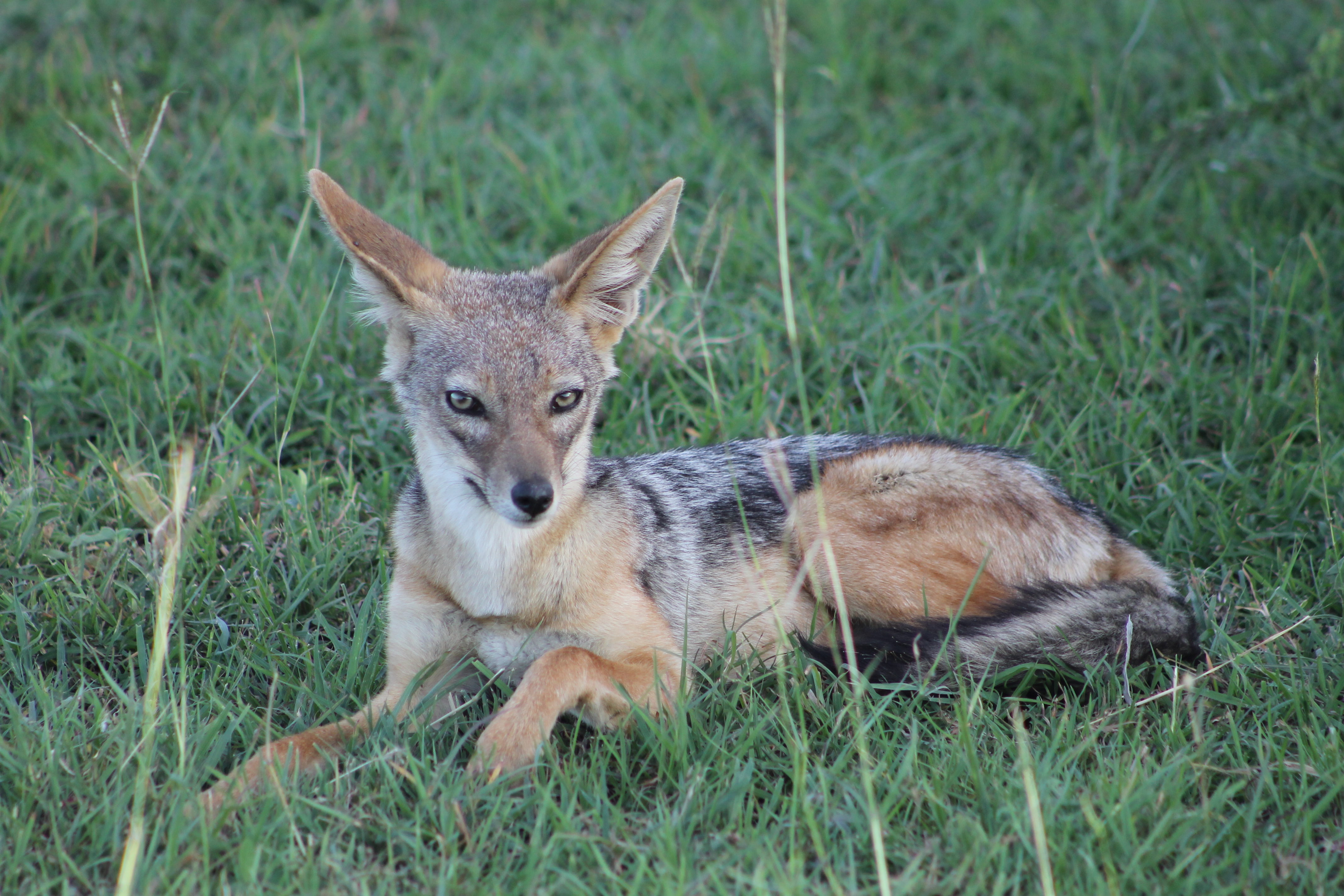
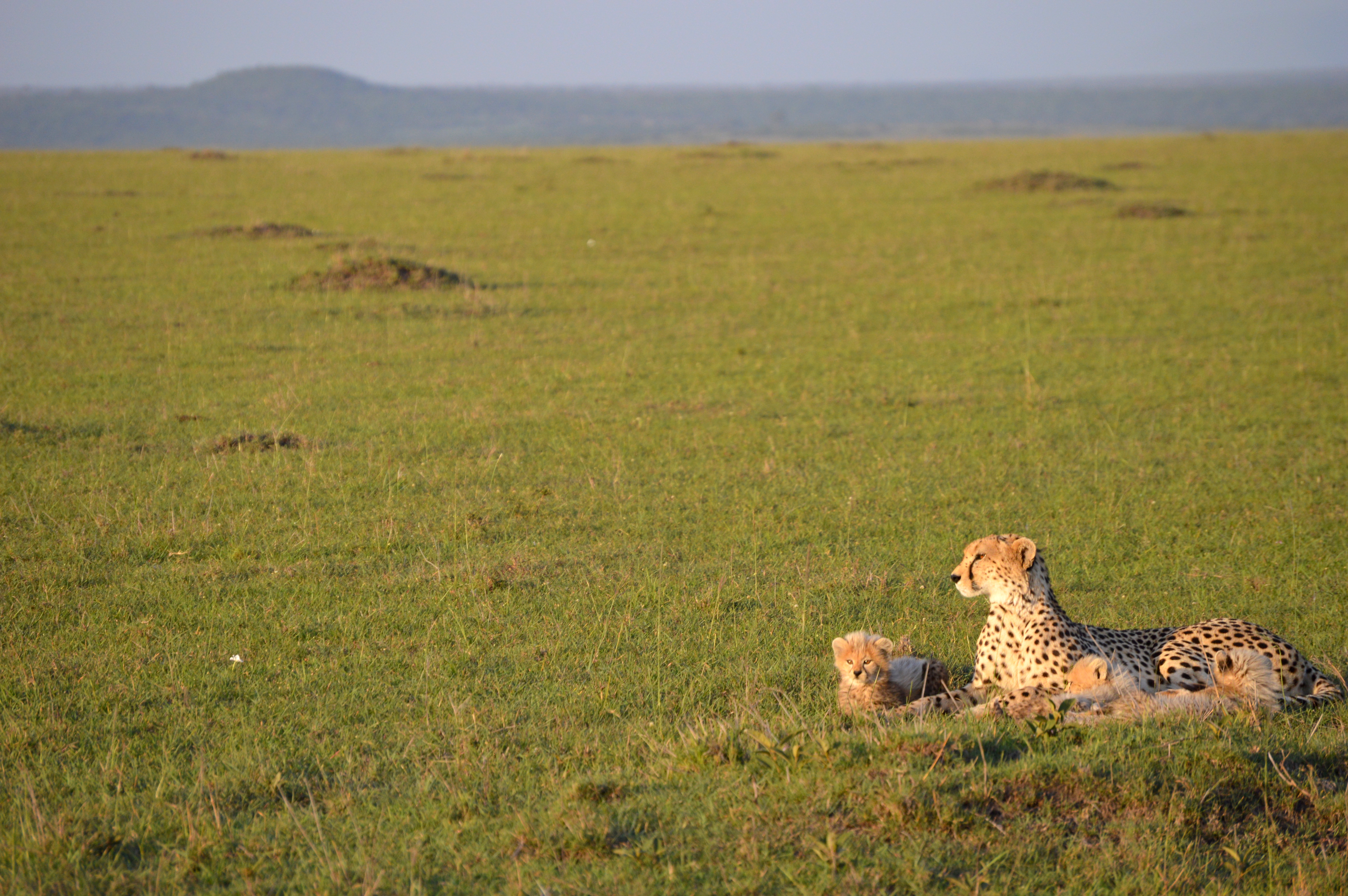
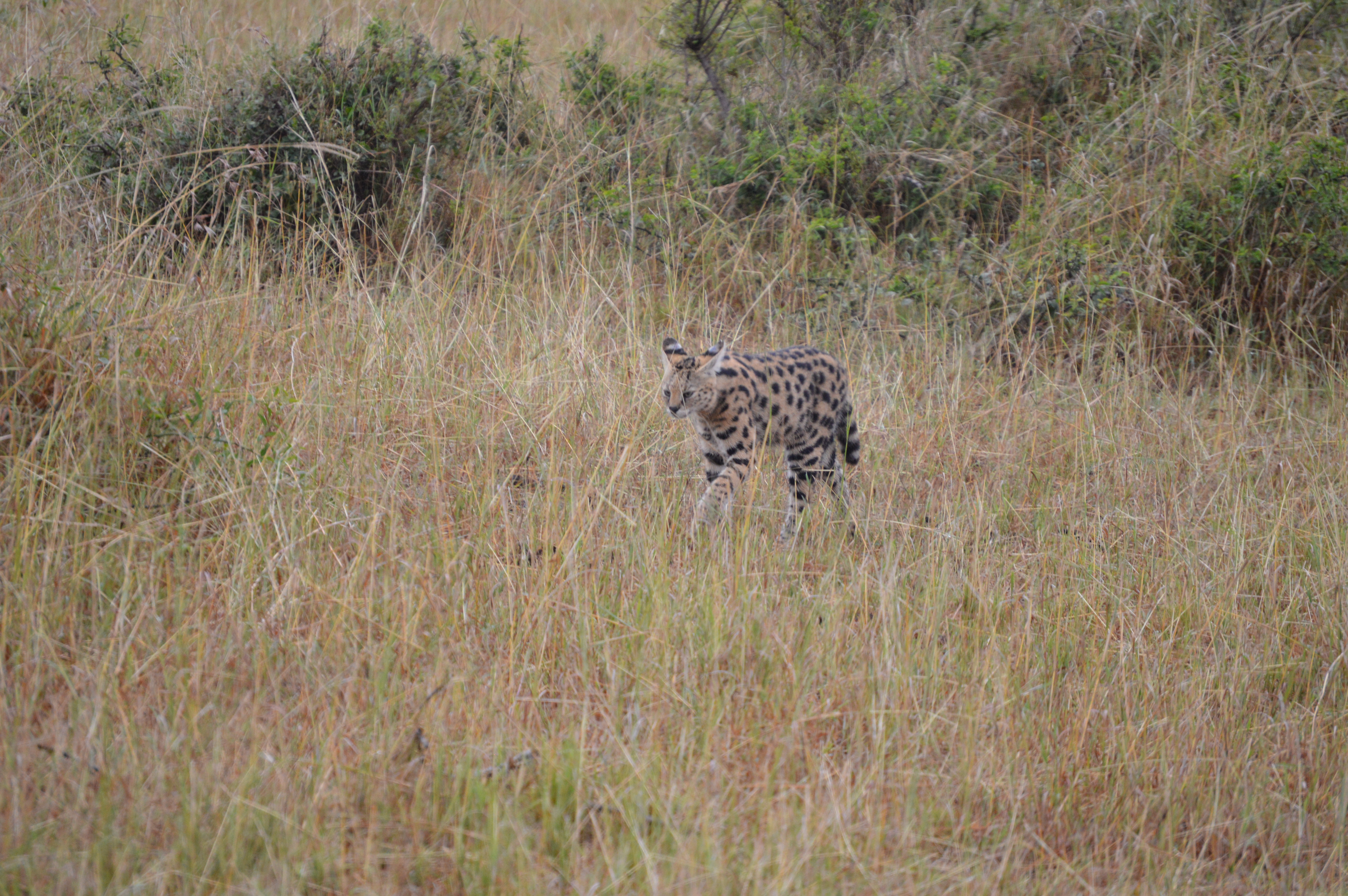
Because of the blatant disturbance, I was curious how wildlife were responding inside the Reserve. Upon my return to the States and immediate start of graduate school, I connected with Dave Green, a PhD student in Kay’s lab (at that time), who spent most of his PhD researching human disturbance on widlife. He along with Kay and Gary Roloff had designed and conducted a distance sampling study between 2012 and 2014 to estimate the abundance of wildlife within the Reserve. Here are photos of a few carnivore species seen during surveys.
As a novice in quantitative ecology, this was my first opportunity to get my feet wet developing a hierarchical model. After chatting with Dr. Beth Gardner about multispecies distance sampling, I dove into developing my first model. It didn’t take me long to get my first JAGS model running, but it wasn’t until 3.5 years later that this project finally led to a publication. My struggle to climb the learning curve of scientific writing and publication was loooooooong, and I commend Elise for her persistance in slogging through the 20+ drafts that it took!
Our main finding, unsurprisingly, was that the effect of passive enforcement of wildlife regulations and resulting human disturbance varied across the carnivore community. Some species (e.g., spotted hyena, black-backed jackal) were more abundant in the presence of disturbance while others (e.g., bat-eared fox, lion) were not. A reduction in lion abundance due to conflicts with humans may be allowing for hyenas and jackals to flourish in the absence of competition. Another hypothesis is that these two species are easily adjusting/adapting to human activities. Either way, communities often do not respond uniformly to humans or the environment, as such it is important to consider all species for both conservation and wildlife management.
This was an extremely beneficial project for me as a new PhD student! Determination, persistence and a few technical pieces that I had to learn along the way made this publication possible. If you’re interested in the statistical side of this project, which I hope you are, keep reading below. And if not… stay tuned for future project blogs!
Matthew Farr farrmat1@msu.edu
To read the actual publication click here.
To return to recent post click here.
Modeling Breakdown
Most of my work for this paper was both estimating the abundance of multiple carnivore species and measuring the effect of management regimes (disturbed vs undisturbed) on the entire carnivore community. We based this off Sollmann et al. 2016.
We used JAGS (Just Another Gibbs Sampler; Plummer 2003) to estimate parameters.
Component 1: Binomial-Poisson Mixture
The first component of this model is a binomial-Poisson mixture:
\[n_{t,j,s} \sim binomial(N_{t,j,s}, p_{t,j,s})\] \[N_{t,j,s} \sim Poisson(\lambda_{t,j,s})\] \(n_{t,j,s}\) is the recorded number of groups (for non-solitary species; more on this later) or counts (solitary species) during replicate \(t\) of transect \(j\) for species \(s\). This is data! \(N_{t,j,s}\) is the latent number of groups (non-solitary) or abundance (solitary), \(p_{t,j,s}\) is detection probability, and \(\lambda_{t,j,s}\) is the expected number of groups (non-solitary) or abundance (solitary).
Here is the code:
n[t,j,s] ~ dbin(N[t,j,s], pcap[t,j,s])
N[t,j,s] ~ dpois(lambda[t,j,s])
The binomial part of this mixture is to link what we see/observe in the field to the actual biological process by accounting for imperfect detection. The second part of the mixture is accounting for stochasticity in latent abundance (or number of groups) by describing it as a random Poisson variable.
Component 2: Imperfect Detection & Distance Sampling
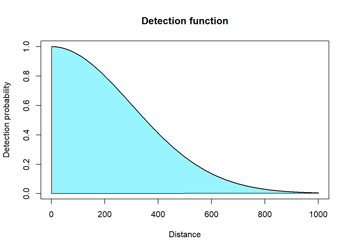
This first component is similar to an N-mixture model, but instead of detection probability being estimated from repeated surveys, it is estimated by a detection function using recorded distances. A variety of detection functions exist (Buckland et al. 1993), but they all have one trait in common, which is that detection probability descreases as a function of distance from the transect.
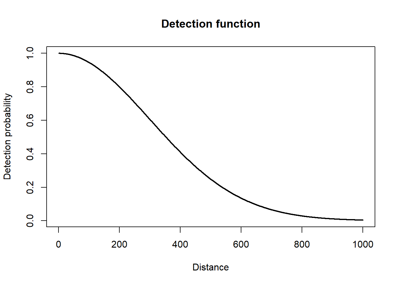
To calculate detection probability you integrate the detection function to find the area under the curve.
However, we find it more convenient to approximate this integral using distance bins (i.e., multiple rectangles).
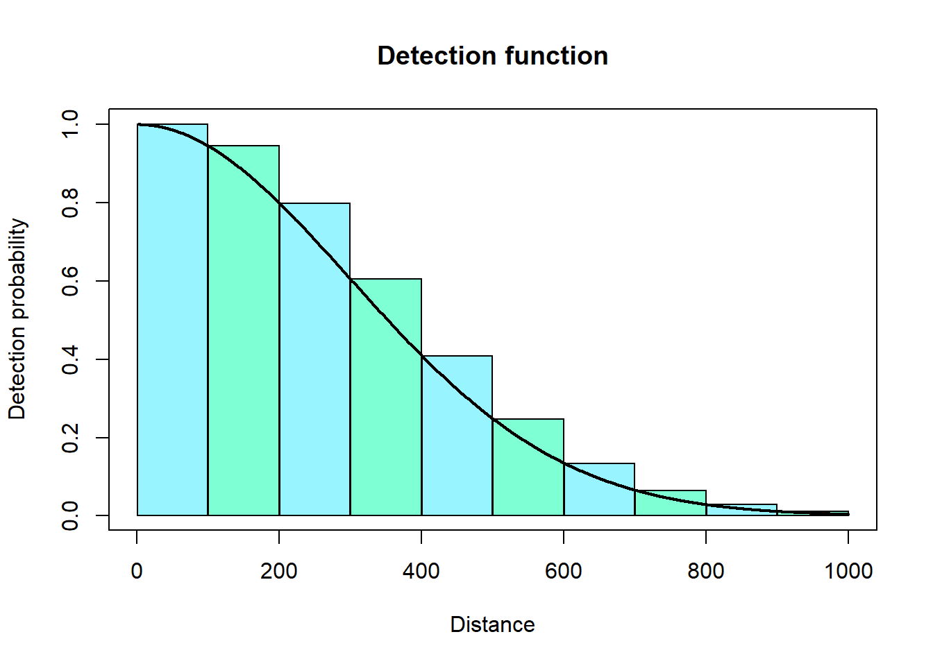
We can then sum up the areas of these rectangles to approximate the area under the curve. The code for this looks like:
g[k,t,j,s] <- exp(-mdpt[k]*mdpt[k]/(2*sigma[j,s]*sigma[j,s]))
pi[k,t,j,s] <- v/B
f[k,t,j,s] <- g[k,t,j,s] * pi[k,t,j,s]
Here g is the height of each rectangle k (t = rep, j = site, s = species) and pi is the width of each rectangle. mdpt[k] is the distance at the midpoint of each class, which is data. sigma is the scale parameter of the half-normal distribution, which we are trying to estimate. v is the length of each distance class (the same for each of the distance classes in our case). B is the transect half-width. We can then sum f up as follows:
pcap[t,j,s] <- sum(f[1:nD,t,j,s])We now need to link these rectangles to our model to be able to estimate them. We do that by splitting our observations, \(n_{t,j,s}\), into each distance class \(k\) giving us \(y_{k,t,j,s}\). The vector of observation across distance classes, \(\mathbf{y_{t,j,s}}\), is the realization of a multinomial distribution: \[\mathbf{y_{t,j,s}} \sim multinomial(n_{t,j,s}, \mathbf{\pi^c_{t,j,s}})\] \(\mathbf{\pi^c_{t,j,s}}\) is the vector of detection probabilities at each distance class (not the same pi as above in the code). The key here is that \(\mathbf{y_{t,j,s}}\) and \(n_{t,j,s}\) are data, so we can easily estimate \(\mathbf{\pi^c_{t,j,s}})\).
We use the categorical distribution within JAGS instead of the multinomial as it is more flexible (See Kéry & Royle 2016, pg. 453). The code for this looks like:
dclass[i] ~ dcat(fc[1:nD, rep[i], site[i], spec[i]])This links the distance for each observation to the conditional detection probability, fc. fc is the area of the rectanlge divided by the total area under the curve:
fc[k,t,j,s] <- f[k,t,j,s]/pcap[t,j,s]Component 3: Group Size
The next component of our model is for group sizes. Often we see individuals of a certain species within a group. These observations violate the assumption of independence. Thus we aggregate these observations by referring them as a group with a group size greater than 1. We can then model the group sizes separately to estimate an average group size and mulitply it by the number of groups to derive abundance. The code for group sizes is:
gs[i] ~ dpois(gs.lambda[s.rep[i], s.site[i], s.spec[i]]) T(1,)gs[i] is the observed group size for a specific observation. We then connect this to the replicate, site, and species. gs.lambda is the average group size for a specific replicate, site, and species.
Component 4: Linear Predictors
We now have the basic distance sampling structure and can move on to estimating variation in expected abundance (or number of groups). We use the log-link function and a linear predictor made up of covariates explaining variation in abundance.
lambda[t,j,s] <- exp(alpha0[s] + ...)We can also model variation in group size:
gs.lambda[t,j,s] <- exp(beta0[s] + ...)Or detection probability:
sigma[j,s] <- exp(gamma0[s] + ...)Component 5: Community Hyper-distributions
To make this a multispecies model, we link parameters within each of the linear predictors above using a random effect by species. We allow for each parameter to have a common or community hyper-distribution with corresponding hyper-parameters (e.g., \(\alpha0_s \sim Normal(\mu_{\alpha0}, \sigma_{\alpha0}^2)\)). Using alpha0 as an example we code this as:
alpha0[s] ~ dnorm(mu_a0, tau_a0)

mu_a0 ~ dnorm(0, 0.01)
tau_a0 ~ dgamma(0.1, 0.1)
sig_a0 <- 1/sqrt(tau_a0)
This allows information between species to be shared, but we still have species-specific estimates of each parameter.
Miscellaneous: Negative Binomial as Poisson-gamma mixture
A miscellaneous topic that I would like to address is the specification of the negative binomial as a Poisson-gamma mixture. We first used a negative binomial for both abundance/number of groups and group size to account for overdispersion. We use a Poisson-gamma mixture, which is an alternate specification of the negative binomial. The JAGS built-in dnegbin uses the classic specification, but the Poisson-gamma mixture is more convenient for our use. The code for this is:
N[i] ~ dpois(lambda[i]*rho[i])
rho[i] ~ dgamma(r, r)
r ~ dgamma(0.1, 0.1)
rho[i] is our dispersion parameter, which is the realization of a gamma distribution. For more information see Greene (2008) or this forum on sourceforge.net.
Literature Cited
Buckland, S.T., Anderson, D.R., Burnham, K.P. & Laake, J.L. (1993) Distance Sampling: Estimating Abundance of Biological Populations. Oxford University Press, Oxford.
Kéry, M. & Royle, J.A. (2016) Applied hierarchical modeling in ecology: Analysis of distribution, abundance and species richness in R and BUGS (volume 1 – prelude and static models), Elsevier, Amsterdam.
Plummer, M. (2003) JAGS: A program for analysis of Bayesian graphical models using Gibbs sampling. Proceedings of the 3rd International Workshop on Distributed Statistical Computing. Vienna, Austria.
Sollmann, R., Gardner, B., Williams, K.A., Gilbert, A.T. & Veit, R.R. (2016) A hierarchical distance sampling model to estimate abundance and covariate associations of species and communities. Methods in Ecology and Evolution, 7, 529–537.